6. 反応速度式の関数でODEを解く方法¶

odeソルバーはNetworkModelを受け入れますが、 ode.ODESimulatorはそのモデルクラスode.ODENetworkModelと ode.ODEReactionRuleを機能拡張のために所有しています。これらのクラスのインタフェースは ModelクラスとReactionRuleとほとんど同じです。ここでは、特に ode.ODERatelawに関するodeに特有の使用法について説明します。

In [1]:

%matplotlib inline
from ecell4 import *

しかし、ode における反応速度式のサポートはまだ開発中の状態です。一部の関数は、将来廃止される可能性があります。現在、反応速度式を有効にするには、オプション ecell4.util.decorator.ENABLE_RATELAWを次のように有効にする必要があります：

In [2]:

util.decorator.ENABLE_RATELAW = True

6.1. ode.ODEReactionRule¶

ode.ODEReactionRuleはReactionRuleとほぼ同じメンバーを持っています。

In [3]:

rr1 = ReactionRule()
rr1.add_reactant(Species("A"))
rr1.add_reactant(Species("B"))
rr1.add_product(Species("C"))
rr1.set_k(1.0)
print(len(rr1.reactants()))  # => 2
print(len(rr1.products()))  # => 1
print(rr1.k())  # => 1.0
print(rr1.as_string())  # => A+B>C|1

2
1
1.0
A+B>C|1

In [4]:

rr2 = ode.ODEReactionRule()
rr2.add_reactant(Species("A"))
rr2.add_reactant(Species("B"))
rr2.add_product(Species("C"))
rr2.set_k(1.0)
print(len(rr2.reactants()))  # => 2
print(len(rr2.products()))  # => 1
print(rr2.k())  # => 1.0
print(rr2.as_string())  # => A+B>C|1

2
1
1.0
A+B>C|1

共通のメンバーに加えて、 ode.ODEReactionRuleは各Speciesの化学量論的係数を格納することができます：

In [5]:

rr2 = ode.ODEReactionRule()
rr2.add_reactant(Species("A"), 1.0)
rr2.add_reactant(Species("B"), 2.0)
rr2.add_product(Species("C"), 2.5)
rr2.set_k(1.0)
print(rr2.as_string())

A+2*B>2.5*C|1

次のように係数にアクセスすることもできます。

In [6]:

print(rr2.reactants_coefficients())  # => [1.0, 2.0]
print(rr2.products_coefficients())  # => [2.5]

[1.0, 2.0]
[2.5]

6.2. ode.ODERatelaw¶

ode.ODEReactionRuleはode.ODERatelawにバインドされます。 ode.ODERatelawは与えられたSpeciesの値に基づいて導関数（フラックスまたは速度）を計算する関数を提供します。 ode.ODERatelawMassActionはode.ODEReactionRuleにバインドされたデフォルトのクラスです。

In [7]:

rr1 = ode.ODEReactionRule()
rr1.add_reactant(Species("A"))
rr1.add_reactant(Species("B"))
rr1.add_product(Species("C"))
rl1 = ode.ODERatelawMassAction(2.0)
rr1.set_ratelaw(rl1)  # equivalent to rr1.set_k(2.0)
print(rr1.as_string())

A+B>C|2

ode.ODERatelawCallbackは、フラックスを計算するためのユーザ定義関数を有効にします。

In [8]:

def mass_action(reactants, products, volume, t, rr):
    veloc = 2.0 * volume
    for value in reactants:
        veloc *= value / volume
    return veloc

rl2 = ode.ODERatelawCallback(mass_action)
rr1.set_ratelaw(rl2)
print(rr1.as_string())

A+B>C|mass_action

bound関数は5つの引数を受け入れ、浮動小数点を速度として返す必要があります。第1および第2のリストは、それぞれ反応物および生成物のそれぞれの値を含みます。化学量論係数にアクセスする必要があるときは、引数に rr（ode.ODEReactionRule）を使います。

ラムダ関数も利用可能です。

In [9]:

rl2 = ode.ODERatelawCallback(lambda r, p, v, t, rr: 2.0 * r[0] * r[1])
rr1.set_k(0)
rr1.set_ratelaw(rl2)
print(rr1.as_string())

A+B>C|<lambda>

6.3. ode.ODENetworkModel¶

ode.ODENetworkModelはReactionRuleと ode.ODEReactionRuleの両方を受け入れます。 ReactionRuleは暗黙的に変換され、ode.ODEReactionRuleとして保存されます。

In [10]:

m1 = ode.ODENetworkModel()
rr1 = create_unbinding_reaction_rule(Species("C"), Species("A"), Species("B"), 3.0)
m1.add_reaction_rule(rr1)
rr2 = ode.ODEReactionRule(create_binding_reaction_rule(Species("A"), Species("B"), Species("C"), 0.0))
rr2.set_ratelaw(ode.ODERatelawCallback(lambda r, p, v, t, rr: 0.1 * r[0] * r[1]))
m1.add_reaction_rule(rr2)

ode.ODENetworkModel中のode.ODEReactionRuleのリストには、モデルのメンバー reaction_rules（）を介してアクセスできます。

In [11]:

print([rr.as_string() for rr in m1.reaction_rules()])

['C>A+B|3', 'A+B>C|<lambda>']

最後に、次のように他のソルバーと同じ方法でシミュレーションを実行できます。

In [12]:

run_simulation(1.0, model=m1, y0={'A': 60, 'B': 60})

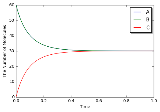
Python のデコレータを使用したモデリングは、レート（浮動小数）の代わりに関数を指定することによっても利用できます。浮動小数点数が設定されている場合、それは質量作用反応の運動速度であると仮定されますが、一定速度ではありません。

In [13]:

with reaction_rules():
    A + B == C | (lambda r, *args: 0.1 * reduce(mul, r), 3.0)

m1 = get_model()

For the simplicity, you can directory defining the equation with Species names as follows:

In [14]:

with reaction_rules():
    A + B == C | (0.1 * A * B, 3.0)

m1 = get_model()

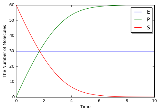
反応物や生成物としてリストアップされていないSpeciesを（速度則中で）呼び出すと、自動的に酵素としてリストに追加されます。

In [15]:

with reaction_rules():
    S > P | 1.0 * E * S / (30.0 + S)

m1 = get_model()
print(m1.reaction_rules()[0].as_string())

S+E>P+E|((1.0*E*S)/(30.0+S))

ここで式中のEは、反応物および生成物リストの両方に付加されます。

In [16]:

run_simulation(10.0, model=m1, y0={'S': 60, 'E': 30})

Speciesの名前の誤字に注意してください。タイプミスをした場合、それは意図せず新しい酵素として認識されてしまいます：

In [17]:

with reaction_rules():
    A13P2G > A23P2G | 1500 * A13B2G  # typo: A13P2G -> A13B2G

m1 = get_model()
print(m1.reaction_rules()[0].as_string())

A13P2G+A13B2G>A23P2G+A13B2G|(1500*A13B2G)

酵素の自動宣言を無効にしたい場合は、 util.decorator.ENABLE_IMPLICIT_DECLARATIONを無効にしてください。その値が Falseの場合、上記の場合はエラーが発生します：

In [20]:

util.decorator.ENABLE_IMPLICIT_DECLARATION = False

try:
    with reaction_rules():
        A13P2G > A23P2G | 1500 * A13B2G
except RuntimeError as e:
    print(repr(e))

util.decorator.ENABLE_IMPLICIT_DECLARATION = True

RuntimeError('unknown variable [A13B2G] was used.',)

E-Cell4は、生化学反応ネットワークのシミュレーションに特化していますが、合成反応ルールを使用することで、常微分方程式を直感的に変換することができます。たとえば、Lotka-Volterraの式は次のようになります。

$\frac{dx}{dt} = Ax - Bxy\\\frac{dy}{dt} = -Cx + Dxy$

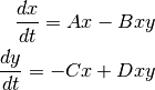
ここで $A=1.5, B=1, C=3, D=1, x(0)=10, y(0)=5$ は以下のように解かれます。

In [19]:

with reaction_rules():
    A, B, C, D = 1.5, 1, 3, 1

    ~x > x | A * x - B * x * y
    ~y > y | -C * y + D * x * y

run_simulation(10, model=get_model(), y0={'x': 10, 'y': 5})

6.4. 速度則における参照について¶

ここで、速度則の定義の詳細を説明します。

第1に、Species で速度則のより単純な定義を使用すると、限られた数の数学関数（例えば exp,log,sin,cos,tan,asin,acos,atan,やpiなど）はブロック外で関数を宣言してもそこで利用できます。

In [20]:

try:
    from math import erf

    with reaction_rules():
        S > P | erf(S / 30.0)
except TypeError as e:
    print(repr(e))

TypeError('a float is required',)

This is because erf is tried to be evaluated agaist S / 30.0 first, but it is not a floating number. In contrast, the following case is acceptable:

In [21]:

from math import erf

with reaction_rules():
    S > P | erf(2.0) * S

m1 = get_model()
print(m1.reaction_rules()[0].as_string())

S>P|(0.995322265019*S)

erf（2.0）、 0.995322265019の結果だけがレート法に渡されます。したがって、上記のレート法は erf関数への参照を持ちません。同様に、外部に宣言された変数の値は受け入れ可能ですが、参照としては使用できません。

In [22]:

kcat, Km = 1.0, 30.0

with reaction_rules():
    S > P | kcat * E * S / (Km + S)

m1 = get_model()
print(m1.reaction_rules()[0].as_string())
kcat = 2.0
print(m1.reaction_rules()[0].as_string())

S+E>P+E|((1.0*E*S)/(30.0+S))
S+E>P+E|((1.0*E*S)/(30.0+S))

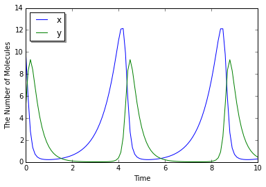
変数の値を変更しても、速度則には影響しません。一方、独自の関数を使用して速度則を定義すると、外部の変数への参照を保持することができます。

In [23]:

k1 = 1.0

with reaction_rules():
    S > P | (lambda r, *args: k1 * r[0])  # referring k1

m1 = get_model()

obs1 = run_simulation(2, model=m1, y0={"S": 60}, return_type='observer')
k1 = 2.0
obs2 = run_simulation(2, model=m1, y0={"S": 60}, return_type='observer')

viz.plot_number_observer(obs1, '-', obs2, '--')

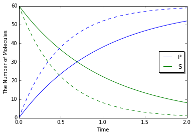
ただし、この場合、パラメータのセットごとに新しいモデルを作成する方が良いです。

In [24]:

def create_model(k):
    with reaction_rules():
        S > P | k

    return get_model()

obs1 = run_simulation(2, model=create_model(k=1.0), y0={"S": 60}, return_type='observer')
obs2 = run_simulation(2, model=create_model(k=2.0), y0={"S": 60}, return_type='observer')
# viz.plot_number_observer(obs1, '-', obs2, '--')

6.5. odeについてより深く¶

ode.ODEWorldでは、各Speciesの値は浮動小数です。しかし、互換性のために、共通メンバ num_moleculesとadd_moleculesはその値を整数とみなします。

In [25]:

w = ode.ODEWorld()
w.add_molecules(Species("A"), 2.5)
print(w.num_molecules(Species("A")))

実数を設定/取得するには、 set_valueとget_valueを使います：

In [26]:

w.set_value(Species("B"), 2.5)
print(w.get_value(Species("A")))
print(w.get_value(Species("B")))

2.0
2.5

デフォルトでは ode.ODESimulatorはROSENBROCK4_CONTROLLERというRosenblock法を使用してODEを解きます。それに加えて、2つのソルバー、 EULERとRUNGE_KUTTA_CASH_KARP54が利用可能です。 ROSENBROCK4_CONTROLLERとRUNGE_KUTTA_CASH_KARP54はエラー制御により時間発展中のステップサイズを適応的に変更しますが、 EULERはこれを行いません。

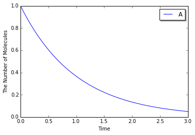
In [27]:

with reaction_rules():
    A > ~A | 1.0

m1 = get_model()

w1 = ode.ODEWorld()
w1.set_value(Species("A"), 1.0)
sim1 = ode.ODESimulator(m1, w1, ode.EULER)
sim1.set_dt(0.01) # This is only effective for EULER
sim1.run(3.0, obs1)

ode.ODEFactoryは、ソルバ型とデフォルトのステップ間隔も受け入れます。

In [28]:

run_simulation(3.0, model=m1, y0={"A": 1.0}, factory=ode.ODEFactory(ode.EULER, 0.01))

下記の例も参照してください。